Backpropagation Through Discrete Nodes

Humans tend to interact with the world through discrete choices, and so they are natural way to represent structure in neural networks. As well, discrete representations are more interpretable, more computationally effecient, and more memory effecient than continuous representations. However, discrete nodes in neural networks are rarely seen because their parameters can’t be learned through backpropagation, due to their non-differential nature. While this problem is usually addressed using alternative training schemes, such as reinforcement learning, a sensible distribution which can be used in standard backpropagation is a preferred solution in many cases.

This blog discusses a recently discovered distribution which can be smoothly annealed into a categorical distribution which represents discrete structure. This trick was discovered simultaneously in two ICLR 2017 conference papers, “Categorical Reparameterization by Gumbel-Softmax” by Eric Jang et al., and “The Concrete Distribution: a Continuous Relaxation of Discrete Random Variables” by Chris Maddison et al. We will refer to this distribution as the Gumbel-Softmax for the remainder of this blog post, though both names could be used interchangeably.

The Problem with Discrete Nodes

To understand why the gradient of discrete operations is undefined, consider the step function:

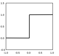
Almost everywhere, a small change in the input results in no change in the output, and so the gradient is zero. For changes where the gradient is not zero, the gradient is infinite and not useful for backpropagation.

A common trick to get around this problem would be to use a continuous approximation to the step function, which has a well defined gradient:

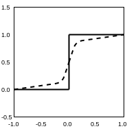
While continuous approximations work reasonably well in some sitations, they fail to produce discrete outputs for “smoother” approximations, and fail to provide useful gradients for “sharper approximations”. Moreover, if a distribution over discrete states is needed there is still no clear solution. While the issues surrounding learning parameters of discrete nodes and learning parameters of distributions over discrete states seem separate, most discrete nodes can be reimagined as samples from a distribution over discrete states.

The Gumbel-Softmax Distribution

Let’s first look at the Gumbel-Max trick, which provides a simple method for draw samples $z$ from a categorical distribution with class probabilites $\pi$. Recall that a Gumbel distribution for the random variable $G$ is defined as:

\begin{equation} G = -log(-log(U)) \end{equation} \begin{equation} U \sim Unif[0,1] \end{equation}

Consider $X$ as a discrete random variable, where:

\begin{equation} P(X = i) \propto \alpha_i \end{equation}

Let $G_i$ be in i.i.d sequence where each $i$ is a standard Gumbel random variable. The Gumbel-Max trick for one-hot encoded vectors is then seen as:

\begin{equation} z = \text{one_hot}(\text{argmax}_i[G_i + log \pi_i]) \end{equation}

In other words, to sample from a discrete categorical distribution we draw a sample of Gumbel noise, add it to $log(\pi_i)$, and use $\text{argmax}$ to find the value of $i$ that produces the maximum. While the choice of Gumbel noise seems arbitrary, it is stable under $max$ operations.

The main problem with this distribution is that the $argmax$ operation is non-differentiable. The trick to resolve this issue, as described in the Gumbel-Softmax and Concrete papers, is to use the $softmax$ function as an approximation to the $argmax$ function:

\begin{equation} y_i = \frac{exp((log(\pi_i)+g_i)/\tau)}{ \sum_{j=1}^{k} exp((log(\pi_j)+g_j)/\tau) } \text{ for } i = 1, …, k \end{equation}

Doing it in TensorFlow

The Gumbel-Softmax distribution is defined tensorflow.contrib as the relaxed one-hot categorical distribution. Consider a 2-category distribution where the probability of choosing category 1 is 0.75, and the probability of choosing category 2 is 0.25. We consider a variety of temperatures:

import tensorflow as tf
from tensorflow.contrib.distributions.python.ops import relaxed_onehot_categorical
sess = tf.InteractiveSession()

dist = relaxed_onehot_categorical.RelaxedOneHotCategorical(temperature=10.0,probs=[0.75,0.25])
dist.sample().eval()

Output:

array([ 0.5162378 ,  0.48376217], dtype=float32)    <- temperature = 10.0
array([ 0.54948032,  0.45051965], dtype=float32)    <- temperature = 5.0
array([ 0.94839412,  0.05160581], dtype=float32)    <- temperature = 1.0
array([ 0.9964357 ,  0.00356426], dtype=float32)    <- temperature = 0.1
array([ 1.,  0.], dtype=float32)                    <- temperature = 0.001

We notice that as the temperature increases, the expected value converges to a uniform distribution over the categories. As the temperature decreases, the distribution becomes one-hot and Gumbel-Softmax distribution becomes identical to the categorical distribution.