Images from on High - The SpaceNet Dataset
Dataset Overview
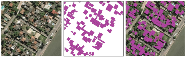
The SpaceNet dataset is a body of 17355 images collected from DigitalGlobe’s WorldView-2 (WV-2) and WorldView-3 (WV-3) multispectral imaging satellites and has been released as a collaboration of DigialGlobe, CosmiQ Works and NVIDIA. The data is composed of multispectral images of cities (200m x 200m patches) with corresponding ground-truth building location data. For each patch, the dataset includes panchromatic, RGB and 8-band multispectral images. Building footprints for each patch (corresponding to a 200m x 200m image) are stored as similarly named GeoJSON files which provide global coordinates that define closed polygons indicating the location and extent of a building within an image. An example of an image and its building footprint ground-truth can be seen below:
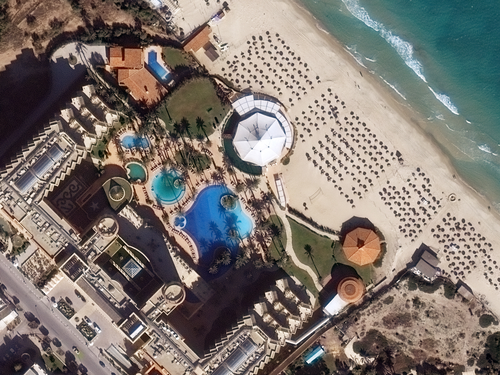
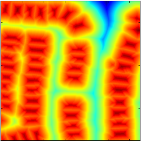
Images come from five cities or “Areas of Interest” (AOI), Rio de Janeiro (AOI_1), Las Vegas (AOI_2), Paris (AOI_3), Shanghai (AOI_4) and Khartoum (AOI_5). Images from Rio de Janeiro were taken with the WV-2 satellite, whereas the remaining cities’ images were taken using the higher resolution WV-3. A high resolution example from the WV-3 is shown here:
The dataset is publicly available through Amazon Web Services (AWS) for free. Download instructions can be found here (SpaceNet on AWS). However, the dataset is readily available for use within the MLRG shared dataset folder: /mnt/data/datasets/SpaceNet. It should be noted that downloading from AWS will require an AWS account which, in turn, requires credit-card information.
Satellite Band Descriptions and Uses
SpaceNet provides panchromatic images which can map to gray-scale images at a resolution per pixel of 0.3m for WV-3 and 0.5m for WV-2. The 8-band, multispectral images include the following bands: Coastal Blue, Blue, Green, Yellow, Red, Red Edge, Near Infrared 1 (NIR1), and Near Infrared 2 (NIR2). Separate RGB images are also provided. The 8-band images on their own have a resolution per pixel of ~1.3m for WV-3 images and ~2m for WV-2 images. However, 8-band and RGB images can have their resolutions increased to their respective satellite’s panchromatic resolution through pansharpening. AOI 2-5 have their full 8-band images pansharpened to ~0.3m of resolution, while AOI 1 has only its RGB images pansharpened to ~0.5m resolution.
Below are some details about the available bands for the SpaceNet dataset and their suggested uses.
The Panchromatic band is a single band image that is sensitive to wavelengths across the visible spectrum, between 450 - 800nm at a resolution of ~0.3m for WV-3 and ~0.5m for WV-2. This band can be used as a gray-scale image of an area and can be used to perform pansharpening for multispectral bands.
The 8-band images have Blue (450 - 510nm), Green (510 - 580nm), and Red (630 - 690nm) bands that cover the majority of the visible spectrum. However, using the raw RGB values from the 8-band images lacks the wavelengths covering yellow, as this is a specific channel in the 8-band images. The 3-band, RGB images have been used in previous building segmentation and identification efforts and have the commonly used RGB channel images covering the visible spectrum.
The Yellow band (585 - 625nm) lies in between the Green and Red bands. The separation of yellow wavelengths, from the usual combination of red, blue and green, provides the ability to assess the “yellowness” of objects directly. This ability may aid in vegetation analysis and novel feature extraction. The Coastal Blue (400 - 450nm) provides a “bluer” blue; these wavelengths of light are absorbed in healthy plants which may allow for further vegetative analysis. Coastal Blue is also weakly absorbed by water, leading to potential uses in bathymetric studies. However, these wavelengths are easily scattered by the atmosphere.
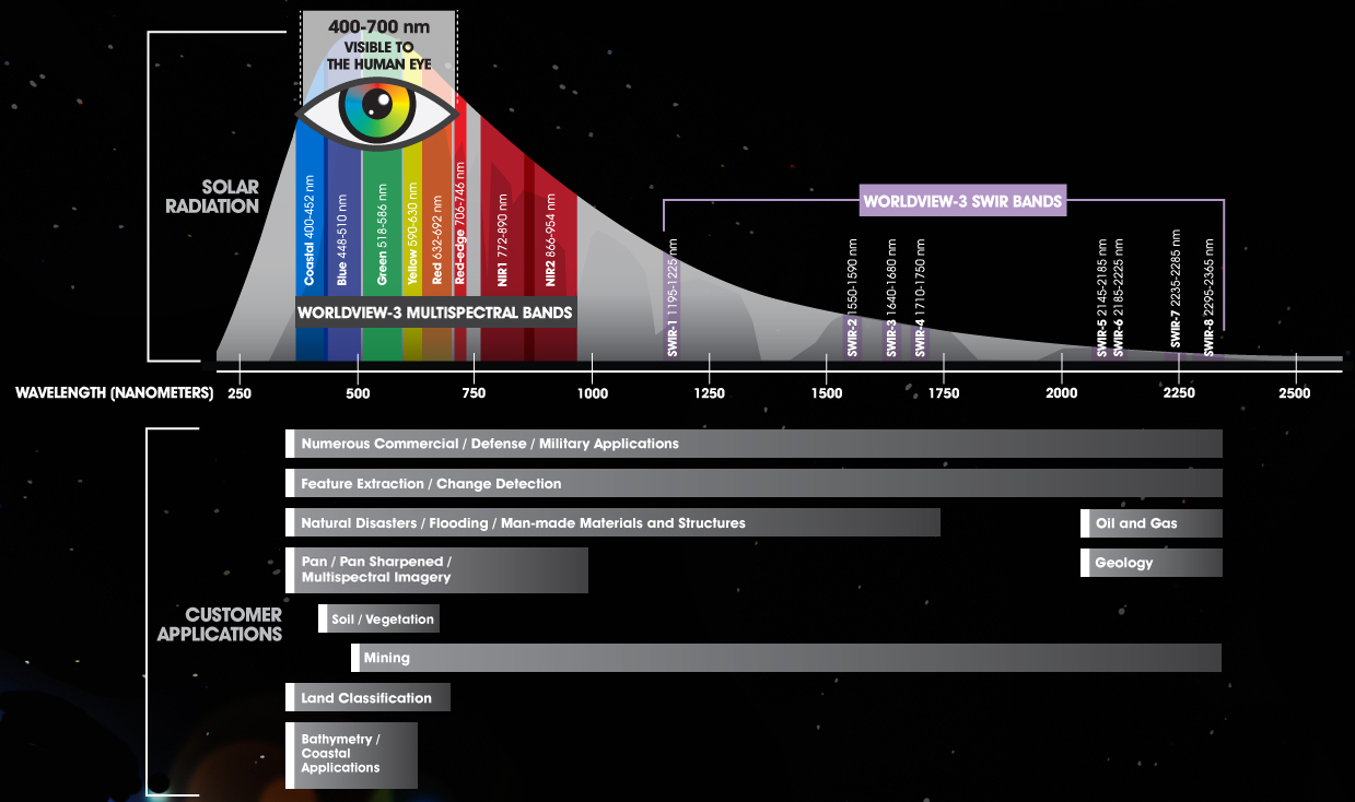
The Red-Edge (705 - 745nm) provides wavelengths of light just beyond the Red wavelengths. The significance of this channel is that Chlorophyll is transparent to wavelengths > 700nm, leading to application for vegetative analysis. The final channels are two Near Infrared (NIR) bands, NIR1 (770 - 895nm), and NIR2 (860 - 1040nm). Both channels can be used to perform NIR spectroscopy, whose applications include investigating plant health, soil conditions and atmospheric analysis. NIR1 can be used to detect moisture content within soil, plant biomass and distinguish water bodies from vegetation. The figure below summarizes the applications of all the bands available with the WV-2 and WV-3 satellites. However, the SpaceNet dataset is limited to the panchromatic, RGB and 8-band channels.
GeoTiff and GeoJSON
GeoTiff images are a special format of image data which incorporate meta-data that can be used for georeferencing an image and how a pixel in the image is mapped to real world distances or vice versa. This information is encoded in the GeoTransform meta-data. An example of of this GeoTransform data can be seen below, as well as it being used to transform from image pixels, to real world map coordinates.
GT = [-115.3022526,2.7000000000043656e-06, 0.0, 36.187967699799998, 0.0, -2.6999999999934342e-06]

Xgeo = GT[0] + Xpixel*GT[1] + Yline*GT[2]
Ygeo = GT[3] + Xpixel*GT[4] + Yline*GT[5]
The 8-band GeoTiff images in the dataset have their channels arranged as rasters in this order, from raster 1 - 8: Coastal Blue, Blue, Green, Yellow, Red, Red Edge, NIR1, NIR2.
The 8-band and RGB images are stored as GeoTiff images which can be read using the python GDAL library. Once loaded, the image rasters must be accessed and copied to a Numpy array. This has already been done for the pansharpened MUL images (AOI 2-5) and the RGB images for AOI 1, further details are below. Panchromatic images are stored as float64 and all other images’ band data are stored using unit16. This convention is maintained in the stored Numpy arrays saved into HDF files.
GeoJSON is simply a JSON file format with a specific hierarchy for geographical data. The primary information of concern for the SpaceNet data is the “geometry” parameter, which contains a set of points defining a closed polygon. The points in the polygon are stored as georeferenced coordinates and require conversion to pixel locations using the inverse operation seen above. Note, the first and last points of a polygon object must be the same point. For more details on GeoJSON please see the GeoJSON Specification. The polygon information is also stored in CSV files.
Example of a GeoJSON file:
{
"type": "FeatureCollection",
"crs": { "type": "name", "properties": { "name": "urn:ogc:def:crs:OGC:1.3:CRS84" } },

"features": [
{ "type": "Feature",
  "properties": { "OBJECTID": 0, "FID_VEGAS_": 0, "Id": 0, "FID_Vegas": 0, "Name": "None", "AREA": 0.000000, "Shape_Leng": 0.000000, "Shape_Le_1": 0.000000, "SISL": 0.000000, "OBJECTID_1": 0, "Shape_Le_2": 74.802692, "Shape_Le_3": 0.000586, "Shape_Area": 0.000000, "partialBuilding": 0.000000, "partialDec": 1.000000 },
  "geometry": { "type": "Polygon", "coordinates":
                          [ [ |--> [ -115.30709085, 36.128288449000024, 0.0 ],
			      |    [ -115.307094415999984, 36.128120471000045, 0.0 ],
			      |    [ -115.307107495999958, 36.128120653000053, 0.0 ],
			Same--|    [ -115.307107764999955, 36.128107957000054, 0.0 ],
			      |    [ -115.307134133354694, 36.128108322332089, 0.0 ],
			      |    [ -115.307135415554143, 36.128289065776833, 0.0 ],
			      |--> [ -115.30709085, 36.128288449000024, 0.0 ] ] ] } },

{ "type": "Feature",
  "properties": { "OBJECTID": 0, "FID_VEGAS_": 0, "Id": 0, "FID_Vegas": 0, "Name": "None", "AREA": 0.000000, "Shape_Leng": 0.000000, "Shape_Le_1": 0.000000, "SISL": 0.000000, "OBJECTID_1": 0, "Shape_Le_2": 70.485000, "Shape_Le_3": 0.000556, "Shape_Area": 0.000000, "partialBuilding": 0.000000, "partialDec": 1.000000 },
  "geometry": { "type": "Polygon", "coordinates": [ [ [ -115.306970441999965, 36.128277326000045, 0.0 ],
						      [ -115.306970441999965, 36.128231828000025, 0.0 ],
						      [ -115.30695475499999, 36.128231828000025, 0.0 ],
						      [ -115.30695475499999, 36.128159838000045, 0.0 ],
						      [ -115.306970441999965, 36.128159838000045, 0.0 ],
						      [ -115.306970441999965, 36.128114916000072, 0.0 ],
						      [ -115.307070266999972, 36.128114916000072, 0.0 ],
						      [ -115.307070266999972, 36.128277326000045, 0.0 ],
						      [ -115.306970441999965, 36.128277326000045, 0.0 ] ] ] } },

...
Example of CSV file containing building footprint polygons:
...
AOI_4_Shanghai_img6626	1	POLYGON ((622.67 109.17 0,573.09 163.68 0,650.0 214.68 0,650.0 127.3 0,622.67 109.17 0))
AOI_4_Shanghai_img6626	2	POLYGON ((-0.0 90.86 0,-0.0 111.26 0,11.63 98.75 0,-0.0 90.86 0))
AOI_4_Shanghai_img6626	3	POLYGON ((414.16 -0.0 0,410.66 -0.0 0,413.13 1.67 0,414.16 -0.0 0))
AOI_4_Shanghai_img6626	4	POLYGON ((369.18 -0.0 0,310.11 -0.0 0,346.45 24.54 0,369.18 -0.0 0))
AOI_4_Shanghai_img6626	5	POLYGON ((166.63 139.95 0,208.18 94.25 0,175.0 72.26 0,143.45 106.96 0,166.63 139.95 0))
AOI_4_Shanghai_img6626	6	POLYGON ((103.7 -0.0 0,82.18 -0.0 0,97.51 9.58 0,105.02 0.82 0,103.7 -0.0 0))
AOI_4_Shanghai_img6626	7	POLYGON ((70.4 -0.0 0,0 0 0,-0.0 65.88 0,28.15 83.48 0,39.96 69.71 0,20.87 57.78 0,70.4 -0.0 0))
...
Converting GeoTiff with GDAL into Numpy Arrays
The following script shows an example of reading in a GeoTiff image into a Numpy array:
import gdal
import Numpy as np

data_root = "/mnt/data/datasets/SpaceNet/"

# Opens GeoTiff as a gdal Dataset which needs Raster information copied to Numpy array
mul_ds = gdal.Open(data_root+"AOI_2_Vegas_Train/MUL-PanSharpen/MUL-PanSharpen_AOI_2_Vegas_img200.tif")


channels = mul_ds.RasterCount
mul_img = np.zeros((mul_ds.RasterXSize, mul_ds.RasterYSize, channels), dtype='uint16')
geoTf   = np.asarray(mul_ds.GetGeoTransform())

for band in range(0, channels):
    mul_img[:,:,band] = mul_ds.GetRasterBand(band+1).ReadAsArray()

# mul_img is a 3-dim Numpy array of size 650x650 with 8 channels stored with dtype uint16
# Channels in order are: Coastal Blue, Blue, Green, Yellow, Red, Red Edge, NIR1, NIR2
Directory Structure
Within the /mnt/data/datasets/SpaceNet directory, the AWS data has been uncompressed into the two following subdirectory templates. The Rio de Janeiro data is formated slightly differently and is missing pansharpened, 8-band, multispectral data, with only RGB channels pansharpened to a resolution of 0.5m. The remaining AOIs all contain similar directory set ups as shown in the second layout.
Subdirectory structure for AOI_1, Rio de Janeiro:
├── AOI_1_Rio_Train
│   ├── 3-Band                   # 3band (RGB) Raster Mosaic for Rio De Jenairo area (2784 sq KM) collected by WorldView-2
│   ├── 8-band                   # 8band Raster Mosaic for Rio De Jenairo area (2784 sq KM) collected by WorldView-2
│   └── processedBuildingLabels
│       ├── 3-Band               # Contains 438 x 406 pixel RGB images pansharpened to 0.5m (200m x 200m)
|       │   └── rio_3_band_label_layers.h5    # *Only in /mnt/data/datasets/SpaceNet HDF file containing Numpy tensors of images last 2 layers are label ground truths
│       ├── 8-band               # Contains 110 x 102 pixel Multi-Spectral images at resolution of ~2m (200m x 200m)
│       │   └── rio_8_band_label_layers.h5   # *Only in /mnt/data/datasets/SpaceNet HDF file containing Numpy tensors of images
│       └── vectordata
│           ├── geojson          # Contains GeoJson labels of buildings for each tile
│           └── summarydata      # Contains CSV with pixel based labels for each building in the Tile Set.
Subdirectory structure for AOI 2-5:
├── AOI_[Num]_[City]_Train
│   ├── geojson
│   │   └── buildings      # Contains GeoJson labels of buildings for each tile
│   ├── MUL                # Contains Tiles of 8-Band Multi-Spectral raster data from WorldView-3
│   ├── MUL-PanSharpen     # Contains Tiles of 8-Band Multi-Spectral raster data pansharpened to 0.3m
│   │    └── [city]_8_band_label_layers.h5 # *Only in /mnt/data/datasets/SpaceNet HDF file containing Numpy tensors of images and last 2 layers are label ground truths
│   ├── PAN                # Contains Tiles of Panchromatic raster data from Worldview-3
│   ├── RGB-PanSharpen     # Contains Tiles of RGB raster data from Worldview-3
│   │    └── [city]_3_band_label_layers.h5 # *Only in /mnt/data/datasets/SpaceNet HDF file containing Numpy tensors of images and last 2 layers are label ground truths
│   └── summaryData        # Contains CSV with pixel based labels for each building in the Tile Set.
Each AOI/city has a different number of images which are listed in their respective folders with the naming convention of [ImageType]\_AOI\_[Num]\_[City]\_img[Index].tif, where the ImageType is the name of the parent directory. The naming convention for the ground truth GeoJSON labels matches the “Index” number of their respective images (either RGB or 8-band) as buildings\_AOI\_[Num]\_[City]\_img[Index].geojson.
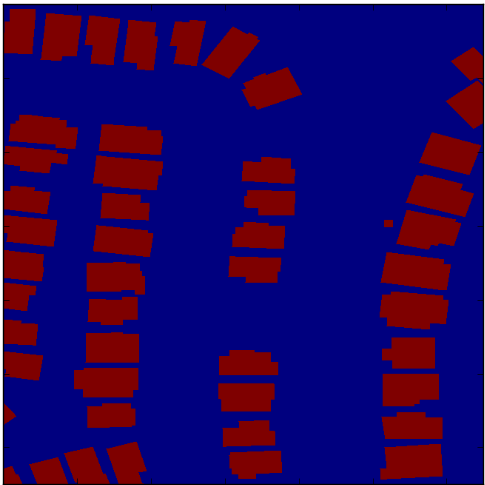
For (potentially) quicker image loading, a HDF file for each city was generated which contains all images stored as 3D Numpy arrays, indexed within the city’s HDF file as img[Index]. Each image has 2 additonal layers which are the binary ground truth for building location as well as the Euclidean distance ground truth, examples of these can be seen below. This convention is open for improvement.
Existing Work & Utilities
Through the SpaceNet Challenge competition and efforts from NVIDIA, there are a number of existing solutions to the problem of identifying buildings in the SpaceNet dataset. The SpaceNet Challenge also provides an evaluation metric for building footprint prediction as well a code for converting GeoTiff images to more common image formats.
SpaceNet Utilities
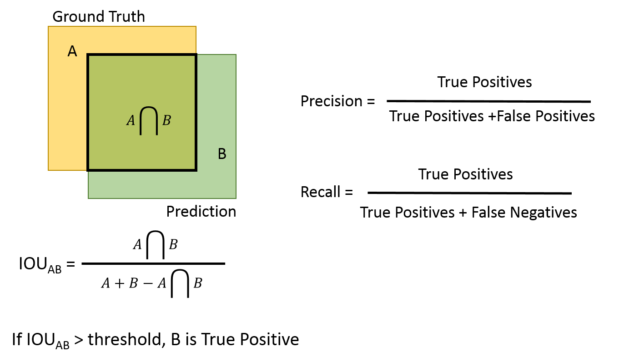
Tools for evaluating building segmentation or detection is provided by here. The metric for evaluation is described in the image below. Conversion scripts are also available in the git repository linked above.
NVIDIA DIGITS
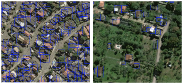
NVIDIA has implemented two solutions to the building detection problem (Exploring the SpaceNet Dataset Using DIGITS), both an object detection and semantic segmentation method. Their object detection method uses a recently added ability for their DIGITS system to perform object detection, called DetectNet. To train their network, the data from Rio de Janeiro was reshaped to be 3-band images 1280 x 1280 such that the bounding boxes that enclosed buildings fell between the pixel range that DetectNet is sensitive to, from 50x50 to 400x400 pixels. The model demonstrated mean precision of 47% and mean recall of 42%. Some examples of results for this method are shown below and further details can be seen in the linked blog post above.
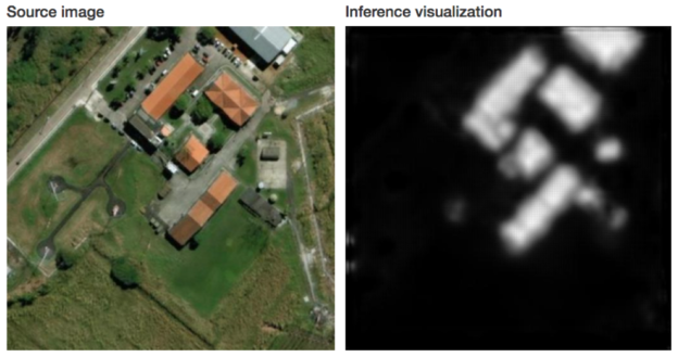
The second method which NVIDIA implemeneted was an instanced segmentation method, which aims to independently classify each pixel individually and then extract segments with common pixel classes that align with individual objects. A fully-convolutional network (FCN) was trained to perform semantic segmentation, with an architecture similar to that of Facebook AI Research’s SharpMask. The SharpMask architecture refines coarse segmentation results by re-feeding results through earlier layers (i.e., features) in the network. Further explanation of the SharpMask network can be found here. The labels for segmentation were altered to be a signed distance value applied to each pixel in an image Yuan 2016. This approach assigns positive values to pixels within a building footprint and negative values to pixels outside a building footprint. Those pixels on the edge of a building footprint will have a zero value. There are two advantages to this labeling regime: 1) Boundaries and regions are captured in a single representation and 2) Train via this representation forces networks to incorporate spatial information such as edges and pixels deep within a region versus far out of one. Segmentation results are shown below and further details on this method can be found at the NVIDIA blog post.
First SpaceNet Challenge Solutions
The SpaceNet challenge endeavors to find solutions to the building segmentation problem through an open competition. As of the date of writing (April 2017), there is a currently active second round for the SpaceNet challenge. The top five best performing models from the first SpaceNet challenge are openly available, SpaceNet Challenge Building Detector winning solutions. Further details on the SpaceNet challenge can be found here.
Links and Resources
- Further images from WorldView-3
- Slide Deck Overview of WorldView-3 Sensors
- WorldView-3 Datasheet
- WorldView-2 Datasheet
- DigiGlobe WorldView-3 Site
- SpaceNet Github with previous challenge winning solutions
- Additional Post on the SpaceNet Challenge
- Exploring the SpaceNet Dataset Using DIGITS
- Automatic Building Extraction in Aerial Scenes Using Convolutional Networks
- Facebook SharpMask